For the past couple of months or so I’ve been programming in Clojure and I really enjoy it.

A good companion in my journey with Clojure has been the Joy of Clojure book, which I simply cannot express how good is.

Michael Fogus and Chris Houser did a really great work in explaining things in a nice and clear way with this book. The book however is probably not appropriate for people who are new to programming in general. It is a great book if you’ve got any prior programming experience and want to deep dive into Clojure.

For novice programmers with no previous or little programming experience I’d probably recommend going with Clojure for the Brave and True. Once you’ve completed it you should get the Joy of Clojure book to get a deeper understanding of the Clojure internals and why certain design decisions have been made, which is where the Joy of Clojure shines.

In this post we are going to see how we can solve one of the classic problems in programming by using Clojure - graph traversal.

Two common ways to represent graphs in computer programs are known as adjacency list and adjacency matrix.

Before we go on and implement our algorithms for graph traversal, let us first create an example graph that we can work with, represented as adjacency list.

(def graph {:A [:B :C]
            :B [:A :X]
            :X [:B :Y]
            :Y [:X]
            :C [:A :D]
            :D [:C :E :F]
            :E [:D :G]
            :F [:D :G]
            :G [:E :F]})

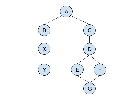
In the Clojure map we’ve created above the keys of the map represent the nodes of our graph and their values represent their neighbors.

This is how our graph looks like represented visually.

Before we go on and implement the graph traversal algorithms we will first define a couple of helper functions to work with.

(defn visited?
  "Predicate which returns true if the node v has been visited already, false otherwise."
  [v coll]
  (some #(= % v) coll))

(defn find-neighbors
  "Returns the sequence of neighbors for the given node"
  [v coll]
  (get coll v))

Depth First Search (DFS)

The following code represents an implementation of a Depth First Search (DFS) algorithm for traversing the graph.

The way that the DFS algorithm works is by first selecting one of the graph nodes as the root and traversing into it’s neighbors as deep as possible before backtracking.

(defn graph-dfs
  "Traverses a graph in Depth First Search (DFS)"
  [graph v]
  (loop [stack   (vector v) ;; Use a stack to store nodes we need to explore
         visited []]        ;; A vector to store the sequence of visited nodes
    (if (empty? stack)      ;; Base case - return visited nodes if the stack is empty
      visited
      (let [v           (peek stack)
            neighbors   (find-neighbors v graph)
            not-visited (filter (complement #(visited? % visited)) neighbors)
            new-stack   (into (pop stack) not-visited)]
        (if (visited? v visited)
          (recur new-stack visited)
          (recur new-stack (conj visited v)))))))

The graph-dfs function is called with an existing graph and a node that we select as the root.

The implementation of the graph-dfs function can be summarized as follows.

We use a stack to store the nodes that we need to process. When we first call the function the only node in the stack is the node we have called our function with. This is the root node that we select for traversing the graph.

Since our DFS implementation is recursive, we also need a base case to indicate when further processing should be stopped. The base case for our graph-dfs function is when the stack is empty we stop further processing and return the sequence of visited nodes.

On each recursion we do the following until the stack is not empty.

1. Get the next node we need to explore by popping out a value from the stack.
2. Get all neighbors of the currently being explored node and filter out the neighbors we have not visited yet.
3. Add the neighbors we have not visited yet to the stack, so we can process them as well.
4. If the currently being explored node has not been visited yet - add it to the list of visited nodes.
5. Recur

We follow steps 1-5 until our stack gets empty at which point we have explored all paths of our graph.

Time to test things out.

user=> (graph-dfs graph :A)
[:A :C :D :F :G :E :B :X :Y]

Note also that our function prefers traversing deeper into the rightmost branch of the neighbors. Should we prefer traversing into the leftmost branch instead we can use the following code for finding the neighbors in the let binding form.

neighbors (-> (find-neighbors graph v) reverse) ;; Prefer leftmost branch when traversing neighbors

Breadth First Search (BFS)

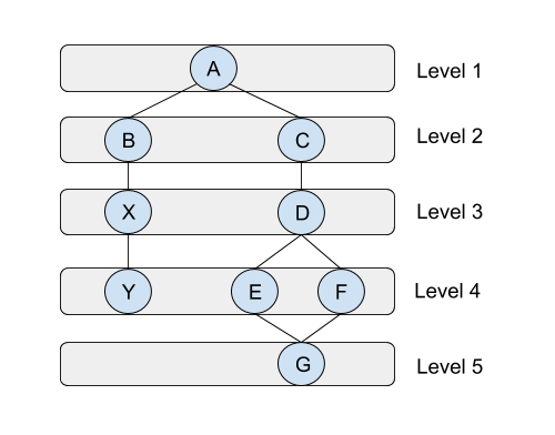
When traversing a graph using Breadth First Search (BFS) we select one of the graph nodes as the root similar to how we do in DFS, and then explore the list of neighbors first before we move on to the next level of neighbors.

Looking at the implementation of the graph-dfs function that we have implemented in the previous section it turns out that we can re-use the code with slight modifications to it in order to turn it into a Breadth First Search algorithm.

For the DFS implementation we have used a stack to store the list of nodes we still need to explore, but if we switch to a queue instead, we can turn our DFS algorithm to a BFS one.

By using a queue instead of a stack we actually delay traversing into the node neighbors deeper, and allows us to explore the list of neighbors in levels instead.

(defn graph-bfs
  "Traverses a graph in Breadth First Search (BFS)."
  [graph v]
  (loop [queue   (conj clojure.lang.PersistentQueue/EMPTY v) ;; Use a queue to store the nodes we need to explore
         visited []]                                         ;; A vector to store the sequence of visited nodes
    (if (empty? queue) visited                               ;; Base case - return visited nodes if the queue is empty
        (let [v           (peek queue)
              neighbors   (find-neighbors v graph)
              not-visited (filter (complement #(visited? % visited)) neighbors)
              new-queue   (apply conj (pop queue) not-visited)]
          (if (visited? v visited)
            (recur new-queue visited)
            (recur new-queue (conj visited v)))))))

Testing our BFS implementation gives us the following results.

user=> (graph-bfs graph :A)
[:A :B :C :X :D :Y :E :F :G]

Works as expected, the result we get is as walking the graph in levels as shown the diagram above.

Dependency Graph

Dependency graphs are useful to represent how some objects relate to each other.

Suppose that we have some kind of a workflow which consists of different steps that need to be executed. In that example workflow a new task should be executed once a previously running one has completed.

Such a workflow can be represented as a dependency graph. Let’s say that we have a task C which depends on B, and B depends on task A.

A visual representation of this dependency graph looks like this.

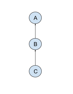
The correct order in which our example workflow would run if we have defined the example graph above would be A -> B -> C.

In order to find the proper evaluation order of a dependency graph we need to perform a topological sort on it.

A good library for working with dependency graphs in Clojure is stuartsierra/dependency. There is also the weavejester/dependency library which is actually a fork of stuartsierra/dependency, but adds support for using a custom comparator during the topological sort, which can be useful in some situations as we will see a bit later.

In this post I am going to use the weavejester/dependency library for our dependency graphs, as we will also make use of the custom comparator function in the next section as well.

Here is how we can construct a dependency graph for our example workflow we talked above.

First, we will define the tasks of our example workflow in a sequence, which will later be reduced to a dependency graph.

user=> (require '[weavejester.dependency :as dep])
nil
user=> (def tasks [{:task :C :depends-on :B}
                   {:task :B :depends-on :A}])
#'user/tasks

This is the function we can use for building the dependency graph for our tasks.

(defn make-dependency-graph
  "Makes a dependency graph from the given collection of tasks"
  [coll]
  (reduce (fn [g x] (dep/depend g (:task x) (:depends-on x)))
          (dep/graph)
          coll))

When adding a new dependency to the graph the library will also take care of catching circular dependencies for us, which is another bonus we get for free.

Let’s create the dependency graph for our tasks.

user=> (def g (make-dependency-graph tasks))
#'user/g

We can also see how our graph looks like if we simply print it. As you can see from the example code below our graph has the proper dependencies set for our tasks.

user=> (require '[clojure.pprint :refer [pprint]])
nil
user=> (pprint g)
{:dependencies {:C #{:B}, :B #{:A}}, :dependents {:B #{:C}, :A #{:B}}}
nil

We can also see the set of immediate or transitive dependencies/dependents of a given graph node as well.

user=> (dep/immediate-dependencies g :C)
#{:B}
user=> (dep/transitive-dependencies g :C)
#{:A :B}
user=> (dep/transitive-dependents g :A)
#{:B :C}

Finally we can derive the proper evaluation order by performing a topological sort of our graph.

user=> (dep/topo-sort g)
(:A :B :C)

The output of the topological order is what we would have expected to see.

Deterministic Topologic Order

The dependency graph presented in the previous section is a simple one, because a given node depends only on some other single node in the graph.

But what about the following dependency graph?

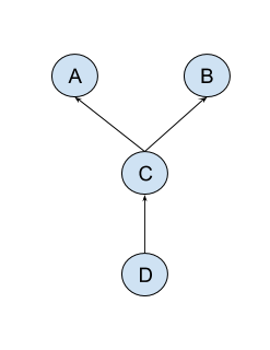
Let’s take a closer look at node C from our graph. Node C depends on both - nodes A and B - but it does not provide any additional information or give preferences which dependency needs to be satisfied first. What node C cares about is that both A and B dependencies are satisfied before it can be evaluated.

So, what would be the topological order of this dependency graph?

Turns out that this dependency graph has two evaluation orders when you perform a topological sort. The first one would be A - B - C - D and the second one would be B - A - C - D.

So, which one is the correct then? Well, they both are! Our dependency graph has two evaluation orders, and they both are equally correct.

But what if you have a requirement that a graph should be topologically sorted in a deterministic way every time we do a topo sort of it?

Can we do that and how? Sure, we can!

In order to resolve the evaluation order of a graph in a deterministic way we can use a custom comparator which will be used when the order is ambiguous.

Suppose that we want to sort nodes based on lexical order when there is any ambiguity during the topological sort.

First, let’s represent our new graph as a sequence of items with their corresponding dependencies.

user=> (def tasks [{:task :C :depends-on :A}
                   {:task :C :depends-on :B}
                   {:task :D :depends-on :C}])

#'user/tasks

This is how our graph looks like when we perform a topological sort without an additional comparator.

user=> (def g (make-dependency-graph tasks))
#'user/g
user=> (pprint g)
{:dependencies {:C #{:A :B}, :D #{:C}},
 :dependents {:A #{:C}, :B #{:C}, :C #{:D}}}
nil
user=> (dep/topo-sort g)
(:B :A :C :D)

As mentioned in the beginning of this section the valid topological orders for our graph are A - B - C - D and B - A - C - D. This means that we will get either of them, but which one will be, we cannot tell for sure.

Looking at the docstring of topo-sort function we see that we can use a custom comparator.

user=> (doc dep/topo-sort)
-------------------------
weavejester.dependency/topo-sort
([graph] [comp graph])
  Returns a topologically-sorted list of nodes in graph. Takes an
  optional comparator to provide secondary sorting when the order of
  nodes is ambiguous.
nil

Let’s create our comparator which will sort nodes based on lexical order. This will give us an evaluation order, which will be deterministic and always resolve the same topological order.

(defn lexical-comparator
  "A comparator which compares x and y in lexical order"
  [x y]
  (compare (name x) (name y)))

And now we can perform the topological order and use our custom comparator as well, which will be used when the order is ambiguous.

user=> (dep/topo-sort lexical-comparator g)
(:A :B :C :D)

Using the lexical-comparator our graph will always resolve in a deterministic way.

We can further expand on this idea and have a more flexible way to specify node preferences when there is ambiguity in the evaluation order.

The latest Clojure project I’ve been working on for internal use consisted of a PostgreSQL backend, a custom configuration language based on EDN and an API with routes exposed as Ring handlers. The goal of the project was to provide a centralized system for describing desired state of components.

Within our organization we have different sub-teams, which manage different components of the infrastructure. For example we have a storage team, a network team, a build team, etc. Each of these teams have different preference and experience when it comes to the Configuration Management systems that they use in order to build and automate stuff. And that is understandable - there is not a single CM tool or system that does everything for everything. One CM system is good at automating network switches, while others have better support for managing OS level stuff, and others are better suited for cloud deployments.

This led us to maintain desired configuration data in different configuration formats, so that they can be consumed by their respective Configuration Management system. Needless to say we ended up with lots of data duplication and fragmentation within the different teams.

For example almost everyone kept a version of the organization NTP servers that we have been using, and this can become an issue whenever you need to update that list, because it’s not easy to keep track or know what or where to look at for all the CM systems that we use - and they are ranging from Puppet, Ansible, Terraform, etc. and even our own internal build and deploy system.

In order to address these issues, we have decided to roll out our own system which can provide all the different teams with a centralized solution for configuration data, which can be consumed by all the different CM systems that we use.

A core requirement of the project was to be able to define the desired state of a component as a self-contained configuration item, or even build a new one from the already existing ones. This led to the implementation of a system similar to inheritance, but designed to work for configuration data only. And with the help of EDN and custom readers we were able to provide people with a way to describe desired configuration in a declarative way, where small configuration snippets can expand to something else. For example we could have a configuration data for a subnet with a start and end IP address, and the system would return back to you a list of available IP addresses within the given range. And this can be even integrated with an IPAM if needed. This kind of solution made our static configuration a bit more dynamic.

Using the custom configuration format based on EDN allows us to standardize on a common format which is used by the different teams, but also allows for describing configuration in a declarative way.

The idea is to make configuration snippets more modular and re-usable in order to build more complex configuration data when needed.

In this system we are able to derive new configuration data by establishing relationships between different components using a parent-child relation, and at the same time a given configuration data may have more than one parent.

Now, the thing with multiple parents is that whenever you resolve all parents you need to make sure that you get a deterministic topological order, because it may happen that both parents contain the same snippets of configuration, so which one resolves before the other also means which one overrides configuration from the other.

The solution we have implemented is similar to the way we have implemented the deterministic lexical order above, but instead on comparing the names of the nodes we are actually comparing the weight of the relationships between the nodes.

For example if we have a node with two parents - we give higher weight to the one we prefer to be sorted before the other. Have a look at the following diagram, which uses weights for the edges.

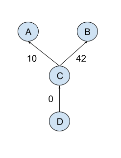
Above dependency graph when topo sorted always resolves to the following evaluation order - B - A - C - D, because B has a path with heigher weight than A, when the two nodes are being compared.

Let’s see how we can create a comparator, which takes into account the weight of the edges. We will first define the relationships we have between the different nodes and their weight.

user=> (def relationships [{:child :C :parent :A :weight 10}
                           {:child :C :parent :B :weight 42}
                           {:child :D :parent :C :weight 0}])
#'user/relationships

Before we implement the weight comparator let’s define a couple of helper functions for working with the relationship collection.

(defn relationship-dependents
  "Returns all nodes which are depending on x"
  [x coll]
  (filter #(= x (:parent %)) coll))

(defn relationship-get
  "Returns the relationship between the given child and parent"
  [child parent coll]
  (-> (filter #(and (= child (:child %)) (= parent (:parent %))) coll)
      first))

We will also need a slightly modified version of the make-dependency-graph function, since the structure of our relationship maps is different.

(defn make-relationship-graph
  "Makes a dependency graph from the given collection of relationships"
  [coll]
  (reduce (fn [g x] (dep/depend g (:child x) (:parent x)))
          (dep/graph)
          coll))

And this is how our weight comparator looks like.

(defn weight-comparator
  "Creates a comparator from the dependency graph of the relationships.
  The comparator is deterministic and will always result in the same
  order when sorting it.

  When there is ambiguity during the topo sort the comparator
  takes into account the weight of the relationships between
  the nodes being compared and their common vertices."
  [coll]
  (fn [x y]
    (let [x-arcs       (->> (relationship-dependents x coll)
                            (map :child)
                            set)
          y-arcs       (->> (relationship-dependents y coll)
                            (map :child)
                            set)
          vertices     (clojure.set/intersection x-arcs y-arcs)
          max-x-weight (->> (map #(relationship-get % x coll) vertices)
                            (map :weight)
                            (apply max))
          max-y-weight (->> (map #(relationship-get % y coll) vertices)
                            (map :weight)
                            (apply max))]
      (compare max-y-weight max-x-weight))))

The weight comparator works as follows. Whenever there is ambiguity between two nodes in the topological order of our graph we find the common vertices of the nodes we compare. Each path between the nodes being compared and their common vertices is then evaluated and the one with the highest weight is chosen.

In the example graph diagram above when we perform topological sort of the graph the comparator is called for nodes A and B. The comparator finds the common vertices of A and B, which in this case is the single node C. Then the following relationship paths are being evaluated - C -> A and C -> B. The one with the heighest weight is between nodes B and C and thus the node B comes before node A in the topological order.

The full evaluation order would then be B - A - C - D.

user=> (def g (make-relationship-graph relationships))
#'user/g
user=> (dep/topo-sort (weight-comparator relationships) g)
(:B :A :C :D)

And this appears to be the correct evaluation order.

The algorithm used by weight-comparator will also work when we compare nodes which have more than one common vertices. In that case all paths are being evaluated and the one with the heighest weight wins.

That is all for now. In another post I intend to write about implementing Dijkstra’s algorithm using Clojure, so stay tuned!